In any field that involves heaps of data and information, details are everything. Load forecasting is no exception. If you’ve spent any amount of time building load forecast models, trying to improve existing ones, conducting out-of-sample tests, etc., then you know these kinds of processes and assessments require paying close attention to the details. “Does that coefficient make sense? What happened in October that made the residual so big? Why does my forecast for Tuesday look a little funky? What is my model missing?” These are some of the questions I find myself asking (or being asked) a lot, and invariably, it forces you to get your hands dirty.
One could argue that the art of building good models is in the details, or as I like to sometimes call them, the residuals. Sure, in-sample fit statistics are useful, but they don’t tell the whole story. Oftentimes overlooked, the residuals can tell a powerful story to those modelers willing to listen. They can reveal outliers and patterns or trends in the data that otherwise might not be easily identified by just looking at the data. And they can give the modeler a sense for what is and isn’t working in their model.
To view a residual chart in MetrixND, you simply go to the Err tab of the model window (press the eyeglasses button) and press the button that looks like a little residual chart on the toolbar. Whether you’re building a model from scratch or polishing off an existing one, this step is a must. What I like to do is take it a step further and plot the residuals against a key variable in my model and see if I’m capturing the right pattern or relationship in my data.
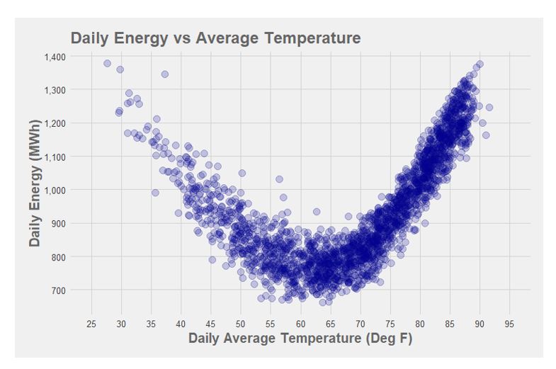
For example, whenever I get asked the question, “Why can’t we just drop average temperature into our linear regression model?” I always show a scatterplot like the one below that illustrates the nonlinear relationship between loads and temperatures.
A simple regression line isn’t going to capture this nonlinearity, but I think this point is really driven home when we put average temperature on the right-hand side of our linear regression equation and then plot the residuals against temperatures.
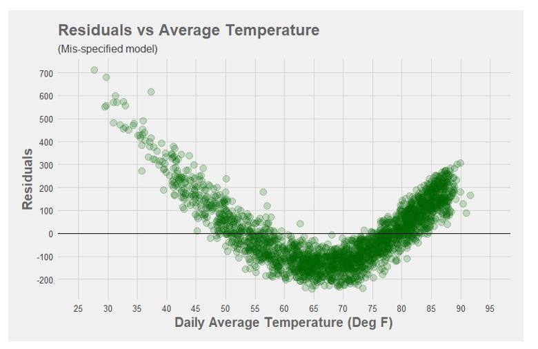
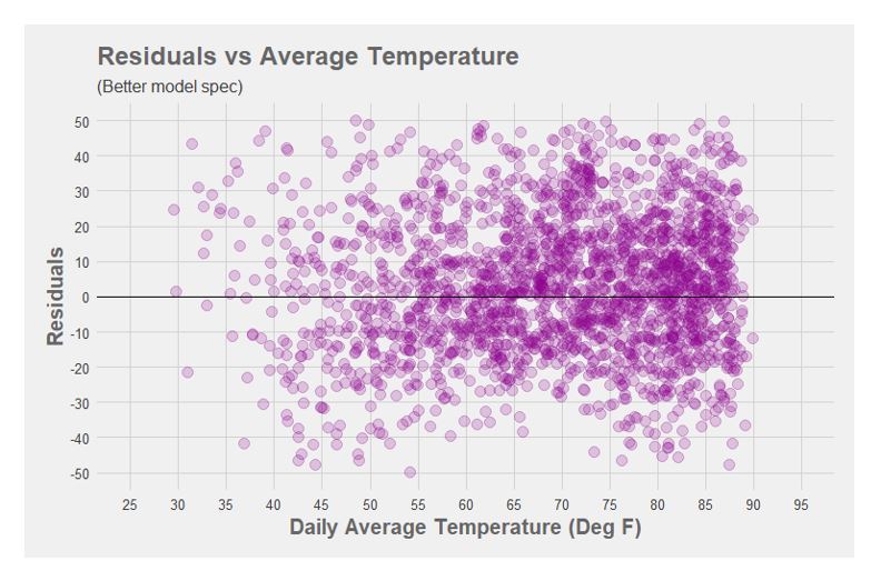
The pattern seen in this scatterplot tells us that our model is mis-specified. The horizontal line at zero is essentially our regression line, which is showing that we’re underpredicting loads at low and high temperatures and overpredicting at mid-range temperatures. If we specify our model correctly, then we would hope to see our residuals reduced to white noise with no discernible pattern (i.e., most of the data hovering around the zero line). Fortunately, when it comes to temperature, we can leverage a polynomial functional form or heating and cooling degree variables to accomplish this.
As the saying goes, “the devil is in the details.” Or as I like to say, “the story is in the residuals.” Perhaps it’s not as catchy, but I think it rings true when it comes to building good load forecast models.
David Simons is a Forecast Consultant with Itron’s Forecasting Division. Since joining Itron in 2013, Simons has assisted in the support and implementation of Itron’s short-term load forecasting solutions for GRTgaz, Hydro Tasmania, IESO, New York ISO, California ISO, Midwest ISO, Potomac Electric Power Company, Old Dominion Electric Cooperative, Bonneville Power Administration and Hydro-Québec. He has also assisted Itron’s Forecasting Division in research and development of forecasting methods and end-use analysis. Prior to joining Itron, Simons conducted empirical research, performed operations analysis and data management for a nonprofit, and lectured in economics at San Diego State University while pursuing his master’s degree. Some of his empirical research includes examining the behavioral factors that influence educational attainment in adolescents and the environmental implications of cross-border integration. Simons received a B.A. in Business Economics from the University of California, Santa Barbara and an M.A. in Economics from San Diego State University.