As forecasters, averaging is something that we do a lot. We like averaging because it helps us filter out much of the noise in our data so that we can confidently identify patterns, trends and causal relationships. But this can get us into trouble if we’re not careful. Specifically, when we do the averaging is crucial—if not executed appropriately, we could filter out valuable information and expose our data and our models to the dangers of aggregation bias.
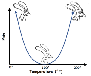
To illustrate, suppose we placed one of our feet in a bucket of water. If the water is at 100 degrees Fahrenheit, this feels like a jacuzzi and we are happy. If the water is zero degrees Fahrenheit, we’re going to be in quite a bit of pain as our foot freezes. On the other hand, if the water is 200 degrees Fahrenheit, our foot is getting scorched—which would also be very painful. In this example, pain is a function of the temperature of the water, and so our pain curve might look something like this.
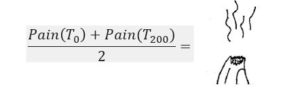
Obviously, the pain function is nonlinear as it has a parabolic shape. Now suppose we stick one foot in the zero degrees Fahrenheit bucket and one foot in the 200 degrees Fahrenheit bucket. To anticipate the level of pain, we need to be careful and think about when to do the averaging. If we average the temperatures first and then compute pain, we would anticipate a nice experience, like stepping into the jacuzzi. Technically:
But we know this can’t be right, because we are really high up on both sides of our pain curve. What we really should do is compute pain first, and then average. This gives us the correct result:
This a classic example of aggregation bias.
To put this idea in the context of electric load forecasting, suppose we have temperature readings from two weather stations—one on the coast and one inland—and we want to combine the data of both stations to build Heating and Cooling Degree Day 65 (HDD65 and CDD65) variables for our forecast model. Since I’m in California, I’m going to use San Francisco and Fresno as an example.
Let’s say on the same day, San Francisco has a temperature of 45 degrees Fahrenheit, while Fresno has a temperature of 85 degrees Fahrenheit (a little drastic, but it could happen). If we first average these temperatures and then compute our CDD65 and HDD65 variables, we’ll get values of 0.0 because the average of 45 and 85 is 65. But, this completely masks the fact that we are probably heating in San Francisco and cooling in Fresno. To get it right, we must first compute the Degree Day variables for each station, and then average to get the combined HDD65 and CDD65 values. If the stations are weighted equally, we would get a CDD65 value of 10 and an HDD65 value of 10—much better values to put into our model. Just like in the pain example, we must do the nonlinear operations first.
The same logic applies for computing normal weather variables for weather-adjusting electricity sales. We want to compute the Heating and Cooling Degree Days for each year first, and then average over the years to calculate a Normal Weather data series. If we average temperature values across years first and then compute Degree Days, we will get normal values that are biased downward, and the weather adjusted sales will be too small.
And this does not just apply to Degree Day calculations. For example, if you use temperature and temperature squared, you should compute the linear and the squared terms for each historical day, then average across days to get the normal values to use in your equations.
The moral of the story is: do the nonlinear operations first before averaging or suffer the pitfalls and pain of aggregation bias.
* Pictures from Matt Groening, How much stress is too much stress, 1990.
David Simons is a Forecast Consultant with Itron’s Forecasting Division. Since joining Itron in 2013, Simons has assisted in the support and implementation of Itron’s short-term load forecasting solutions for GRTgaz, Hydro Tasmania, IESO, New York ISO, California ISO, Midwest ISO, Potomac Electric Power Company, Old Dominion Electric Cooperative, Bonneville Power Administration and Hydro-Québec. He has also assisted Itron’s Forecasting Division in research and development of forecasting methods and end-use analysis. Prior to joining Itron, Simons conducted empirical research, performed operations analysis and data management for a nonprofit, and lectured in economics at San Diego State University while pursuing his master’s degree. Some of his empirical research includes examining the behavioral factors that influence educational attainment in adolescents and the environmental implications of cross-border integration. Simons received a B.A. in Business Economics from the University of California, Santa Barbara and an M.A. in Economics from San Diego State University.